REINFORCE - A Quick Introduction (with Code)
The REINFORCE algorithm is a popular and well-known algorithm in the field of reinforcement learning. It is a type of policy gradient algorithm that is used to optimize the policy or decision-making mechanism in an agent.
The REINFORCE algorithm is used to update the policy based on the gradient of the expected total reward. Unlike other reinforcement learning algorithms, the REINFORCE algorithm does not use value functions to evaluate the quality of a policy, but instead directly optimizes the policy.
- Understanding Monte Carlo Policy Gradients
- How does the REINFORCE algorithm work?
- Implementation of REINFORCE
- Strengths and weaknesses
- Strengths of the REINFORCE algorithm
- Weaknesses of the REINFORCE algorithm
- Comparing with other RL algorithms
- Final Thoughts
Understanding Monte Carlo Policy Gradients
Monte Carlo policy gradients are a type of gradient estimation that uses Monte Carlo methods to estimate the gradient of the expected reward with respect to the policy parameters.
Monte Carlo methods
Broadly speaking, Monte Carlo methods are a group of methods that samples randomly from a distribution to eventually localize to some solution. In the context of RL, we use Monte Carlo methods to estimate the reward by averaging the rewards over many episodes of interaction with the environment.
Monte Carlo Policy Gradients
The Monte Carlo Policy Gradient method is the subset of policy gradient methods where we update the policy parameters after every episode. This is in contrast to Temporal Difference Learning approaches, where the parameters are updated after each step (a.k.a. action). The Monte Carlo approach leads to a more stable (but slightly slower) convergence to the optimal parameters.
How does the REINFORCE algorithm work?
The REINFORCE algorithm works by using the Monte Carlo policy gradient theorem to update the policy in the direction of the maximum expected reward. The algorithm consists of the following steps:
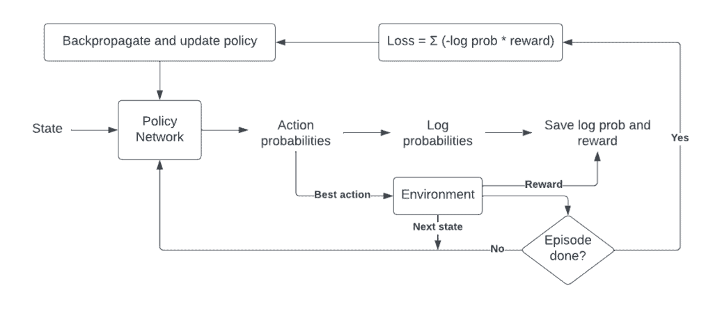 REINFORCE Architecture
A. Observe the state of the environment
The agent first observes the state of the environment and selects an action to take based on its current policy. This is done by sampling from the action probabilities output by the policy network.
B. Take an action and observe the reward
The agent then takes the selected action and receives a reward from the environment.
C. Continue taking actions until the episode ends
The agent continues to take actions as per its policy until a terminal state is reached. Throughout the process, we keep track of the actions taken (or rather the log probabilities of the actions) and the rewards observed.
D. Update the policy
Next, we update the policy. For this, we use the log probabilities from before, scale this by the reward, and directly use the negative of this product as the loss for our policy network (minimizing this negated product is the same as maximizing the reward-weighted log probabilities). Now, we can simply backpropagate through this product to update the policy. Take a look at my blog post on Policy Gradients for a more thorough explanation. You can also check out this video which explains policy gradients in an intuitive way.
E. Repeat the process
We repeat this process for a number of iterations until the policy converges to the optimal policy which maximizes the expected total reward.
Implementation of REINFORCE
 CartPole task provided by OpenAI Gym
The implementation is essentially the same as the one I gave for policy gradients. I will duplicate the implementation here for convenience. Head over to the Policy Gradients blog post for a thorough explanation.
import gym
import numpy as np
import torch
import torch.nn as nn
import torch.optim as optim

# Create the environment
env = gym.make("CartPole-v1")

# Get the state and action sizes
state_size = env.observation_space.shape[0]
action_size = env.action_space.n

# Define the policy function (neural network)
class Policy(nn.Module):
    def __init__(self):
        super(Policy, self).__init__()
        self.fc1 = nn.Linear(state_size, 32)
        self.fc2 = nn.Linear(32, action_size)

    def forward(self, x):
        x = torch.relu(self.fc1(x))
        x = self.fc2(x)
        return torch.softmax(x, dim=-1)

policy = Policy()

# Define the optimizer
optimizer = optim.Adam(policy.parameters(), lr=0.01)

# Define the update policy function
def update_policy(rewards, log_probs, optimizer):
    log_probs = torch.stack(log_probs)
    loss = -torch.mean(log_probs) * (sum(rewards) - 15)
    optimizer.zero_grad()
    loss.backward()
    optimizer.step()

gamma = 0.99

# Training loop
for episode in range(5000):
    state, _ = env.reset()
    done = False
    score = 0
    log_probs = []
    rewards = []

    while not done:
        # Select action
        state = torch.tensor(state, dtype=torch.float32).reshape(1, -1)
        probs = policy(state)
        action = torch.multinomial(probs, 1).item()
        log_prob = torch.log(probs[:, action])

        # Take step
        next_state, reward, done, _, _ = env.step(action)
        score += reward

        rewards.append(reward)
        log_probs.append(log_prob)
        state = next_state

    # Update policy
    print(f"Episode {episode}: {score}")
    update_policy(rewards, log_probs, optimizer)
Strengths and weaknesses
The REINFORCE algorithm is a simple and flexible algorithm that has been widely used in reinforcement learning. However, like all algorithms, it has its strengths and weaknesses.
Strengths of the REINFORCE algorithm
-
Simple and flexible
-
Can handle large state spaces
-
Easy to implement
Weaknesses of the REINFORCE algorithm
-
High variance
-
Slow convergence
-
Sensitive to hyperparameters
Comparing with other RL algorithms
The REINFORCE algorithm is just one of many algorithms used in reinforcement learning. In this section, we will compare the REINFORCE algorithm with other reinforcement learning algorithms.
Comparison with Value-based Methods
Value-based methods, such as Q-Learning and SARSA, estimate the value of taking a particular action in a particular state. Unlike the REINFORCE algorithm, value-based methods do not require a policy representation, making them more sample-efficient. However, value-based methods are less flexible than the REINFORCE algorithm, as they cannot handle complex policies.
Comparison with Actor-Critic Methods
Actor-critic methods, such as A2C and PPO, combine the strengths of both value-based and policy-based methods. Actor-critic methods estimate both the value function and the policy and use the value function as a baseline to reduce the variance of the gradient estimate. Unlike the REINFORCE algorithm, actor-critic methods are more sample-efficient and can handle complex policies.
Comparison with Model-based Methods
Model-based methods, such as Dyna and Model-based RL, use a model of the environment to learn the optimal policy. Unlike the REINFORCE algorithm, model-based methods do not require a policy representation and can handle environments with sparse rewards. However, model-based methods can be more computationally expensive and require more data to learn the model.
Final Thoughts
REINFORCE is often referred to as the simplest version of policy gradients. However, understanding it is important before working up to more complex algorithms.
Hope you found this helpful! Feel free to comment below if you have any questions, or check out my other explanations of RL concepts here.