The Reparameterization Trick - Clearly Explained
The reparameterization trick is an ingenious method to sidestep the challenge of backpropagating through a random or stochastic node within a neural network. This has found prominence, particularly in the context of Variational Autoencoders (VAEs). In this blog post, we will discuss what the reparameterization trick is and what it solves.
- Gaussian Distribution Basics
- Backpropagating Over Randomness
- Reparameterization Trick
- Reparameterization Trick in VAEs
- Additional Resources
- Conclusion
Gaussian Distribution Basics
To comprehend the reparameterization trick fully, it is essential to grasp the fundamentals of the Gaussian distribution, often denoted as $\mathcal{N}(μ,σ)$. This distribution is characterized by two key parameters: the mean ($\mu$), representing the average, and the standard deviation ($\sigma$), governing the spread or width of the distribution.
We can visualize the Gaussian distribution’s behavior by exploring variations in $\mu$ and $\sigma$. When $\mu$ remains constant, altering $\sigma$ results in variations in the width of the distribution. Similarly, adjusting $\mu$ shifts the location of the peak.
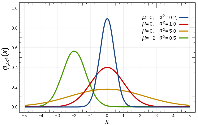 Gaussian Distributions with varying $\mu$ and $\sigma$
Backpropagating Over Randomness
Backpropagation is like a teacher guiding a student to correct mistakes. But when faced with a randomly sampled variable, it’s like the teacher saying, “Figure out how this random outcome influenced your mistake”. Not as straightforward as correcting a regular math problem, right?
Now let’s imagine we have a neural network tasked with learning from data. Say we have a node in our neural networks that samples a variable (let’s call it $z$) from a Gaussian distribution with mean (μ) and standard deviation (σ). In such a case, traditional backpropagation struggles to calculate the derivative since the final output has no idea which inputs resulted in the sampled $z$ variable.
Reparameterization Trick
Enter – the reparameterization trick. This clever technique allows us to sidestep the hurdle of backpropagating over a randomly sampled variable. Instead of leaving randomness inside the network node, we move it outside, making it deterministic.
Following our previous analogy of correcting mistakes, the reparameterization trick is like the teacher saying, “Okay, I see that your studies depend on your concentration and study time. I understand that the background noise may affect your concentration, but the noise is out of our control. So, let’s try to optimize your concentration and study time instead”.
Coming back to neural networks, instead of sampling the random node from a normal distribution with a given mean and variance, we extract the randomness as a separate input that need not be optimized.
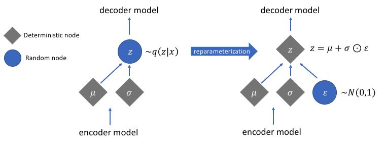 The reparameterization trick
In other words, the reparameterization trick provides a workaround by employing a function (let’s call it $g$) that transforms a known distribution – typically a simple normal distribution with a mean of zero and a standard deviation of one. This function $g$ takes a random variable (often denoted as epsilon $ϵ$) from the known distribution and, by incorporating the mean (mu $μ$) and standard deviation (sigma $σ$), simulates the sampling as if it’s from the desired distribution.
So, instead of the regular definition of z
we define $z$ as
where,
Since $\mu$ and $\sigma$ are the parameters we want to optimize, we don’t want it to be any part of the generation of randomness. Through the above formulation, we remove the necessity of training the parameters for the randomness, since it’s now fixed to $\mu=0$ and $\sigma=1$.
Reparameterization Trick in VAEs
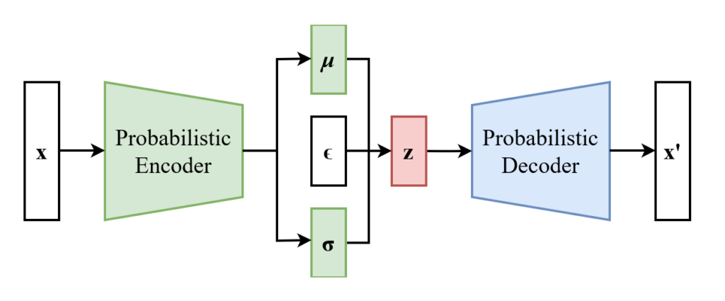 Variational Autoencoder with the Reparameterization Trick
To grasp the significance of the reparameterization trick in Variational Autoencoders (VAEs), let’s first understand the fundamental mechanics of regular autoencoders.
Regular Autoencoders
In a conventional autoencoder, the primary objective is to reconstruct input data faithfully. It consists of an encoder, which compresses the input data into a lower-dimensional representation, and a decoder, which reconstructs the original data from this compressed representation. However, this process doesn’t involve generating new samples; rather, it excels at reproducing the input it was trained on.
Variational Autoencoders (VAEs)
Variational Autoencoders take a different approach. Instead of focusing solely on reconstructing input data, VAEs are designed to generate new samples. The encoder in a VAE, too, compresses input data, but not directly into a latent vector. Instead, the VAE predicts two variables, a mean and a standard deviation (or variance). These two variables are used to sample the latent vector from a Gaussian distribution defined by that mean and standard deviation.
This introduces a layer of uncertainty, as opposed to the deterministic reconstruction of regular autoencoders. The challenge arises when we seek to train such a model using backpropagation, a process that relies on calculating derivatives.
To train the VAE, we need to sample a latent variable ($z$) during the generation process. However, standard backpropagation struggles with random or stochastic processes, hindering our ability to compute accurate derivatives and fine-tune the model effectively.
The Reparameterization Trick
As previously discussed, instead of directly sampling $z$ within the neural network, we introduce a deterministic transformation. We create a function g that takes a random variable (ϵ) sampled from a simple known distribution (typically a normal distribution with mean zero and standard deviation one).
Additional Resources
I have chosen not to dive too deep into the math behind the reparameterization trick and VAEs in this post.
-
For the math behind the reparameterization trick, I recommend this video.
-
For the math behind VAEs, I recommend this video or this blog post.
-
You can also find a good explanation of how the reparameterization trick works in VAEs on this StackOverflow question.
-
If you have the time and want a more thorough, bottom-up explanation of VAEs, I recommend watching lectures 21 and 22 of this playlist of CMU lectures.
Conclusion
Despite what was discussed in this blog post, the applicability of the reparameterization trick is neither limited to VAEs nor to Gaussian distributions. The reparameterization trick may be utilized for backpropagating through a stochastic node of any distribution whose samples can be expressed as a deterministic, differentiable function of its parameters and a fixed source of randomness, through any network. Further, it has favorable properties such as the reduction of variance.
Feel free to take a look at the AI Math section of this blog if you would like to see other articles on mathematical concepts of AI.