Custom Image Classifier with PyTorch - A Step-by-Step Guide
In this article, I’ll explain how to create a custom image classifier using PyTorch in 6 steps:
-
Define the transforms
-
Define the datasets and dataloaders
-
Define the model
-
Define the loss function and the optimizer
-
Train the model
-
Test the model
We’ll discuss each of these steps below. However, if you just want the entire code for the custom image classifier, simply head to the Notebook section at the end of this article where I’ve attached a notebook.
- 1. Define the transforms
- 2. Define the datasets and dataloaders
- 3. Define the Classifier model
- 4. Define the loss function and the optimizer
- 5. Training the classifier model
- 6. Testing the classifier model
- Notebook for Custom Image Classifier
- Conclusion
1. Define the transforms
Transforms refer to the preprocessing and augmentation operations we apply to the dataset before we feed it for training. You can think of the augmentations as a way to add more data to our dataset.

Data augmentations
To use transforms in PyTorch, import the following:
import torchvision.transforms as transforms
Next, you can define the transforms as follows:
transform = transforms.Compose([
    transforms.Resize((128, 128)),
    transforms.RandomHorizontalFlip(p=0.5)
])
The transform variable created above is basically a function. Calling tranform(image) would return an image which is an augmented version of the input image.
You can find a list of all the transforms and their explanations here.
2. Define the datasets and dataloaders
Note: This section assumes that you haven’t split your dataset into train and test (or train, test, and validation). If you’ve already split the dataset, simply create each dataset pointing to the respective folder containing the split of your data. In the below case, I create the dataset pointing to the root folder that has all the images and then I split the dataset after it has been created.
When it comes to creating the dataset, you have two options:
-
Use PyTorch’s ImageFolder class
-
Define a custom dataset
Let’s take a look at both these options.
ImageFolder
To use the ImageFolder class, you must first create the folder structure appropriately.
Your dataset should be a folder that contains a set of sub-folders. Each sub-folder should contain the images belonging to a single class.
For example: Let’s say your dataset is a "cats vs dogs vs rabbits" classifier (very typical, I know). Then, your dataset folder should look like the following:
data/
├─ dog/
│  ├─ dog1.jpg
│  ├─ dog2.jpg
│  ├─ ....
├─ cat/
│  ├─ cat1.jpg
│  ├─ cat2.jpg
│  ├─ ....
├─ rabbit/
│  ├─ rabbit1.jpg
│  ├─ rabbit2.jpg
│  ├─ ....
Now, we can define our dataset using the ImageFolder class of PyTorch.
First, import the class using:
from torchvision.datasets import ImageFolder
Next, define the dataset using:
train_dataset = torchvision.datasets.ImageFolder(root='data', transform=transform)
In the above line,
-
root= path to your dataset root directory -
transform= the transform we defined earlier
Custom Dataset
In the case of the custom dataset, your folder structure can be in any format. You can specify how each image should be loaded and what their label is, within the custom dataset definition. For the sake of consistency, I will show how to create a custom dataset for the folder structure described in the previous section.
A custom dataset class has 3 methods that we need to define. These are the __init__(), __len__(), and __getitem__() methods.
First, let’s import the Dataset class, the function for reading an image, and the enum containing the different image modes (RGB, grayscale, etc.).
from torch.utils.data import Dataset
from torchvision.io import read_image, ImageReadMode
Next, as per the previously mentioned folder structure, the custom dataset class definition can be the following.
import glob
import os


class CustomDataset(Dataset):
    def __init__(self, root_dir, transform):
        self.transform = transform
        self.image_paths = []
        for ext in ['png', 'jpg']:
            self.image_paths += glob.glob(os.path.join(root_dir, '*', f'*.{ext}'))
        class_set = set()
        for path in self.image_paths:
            class_set.add(os.path.basename(os.path.dirname(path)))
        self.class_lbl = { cls: i for i, cls in enumerate(sorted(list(class_set)))}

    def __len__(self):
        return len(self.image_paths)

    def __getitem__(self, idx):
        img = read_image(self.image_paths[idx], ImageReadMode.RGB).float()
        cls = os.path.basename(os.path.dirname(self.image_paths[idx]))
        label = self.class_lbl[cls]

        return self.transform(img), torch.tensor(label)
Note: If your directory has image types other than .png or .jpg, then don’t forget to add it to the list in line 6 of the above snippet.
Finally, you can instantiate the dataset object with the following:
dataset = CustomDataset('data/', transform)
Split the dataset
Let’s first define the ratio by which we want to split the dataset. For this example, I will split the dataset as 80% for the training set, 10% for the test set, and 10% for the validation set.
splits = [0.8, 0.1, 0.1]
Next, we’ll create the list of split sizes:
split_sizes = []
for sp in splits[:-1]:
    split_sizes.append(int(sp * len(dataset)))
split_sizes.append(len(dataset) - sum(split_sizes))
Note: We’re adding the size of the last split separately since there’s a chance that we could lose a few samples to rounding errors when we use the int function. In the above way, all the remaining samples would be added to the list of split sizes.
Finally, we’ll split the dataset using PyTorch’s random_split function:
train_set, test_set, val_set = torch.utils.data.random_split(dataset, split_sizes)
If you would like to specify a different set of transforms for the validation set and test_set, note that random_split returns Subset objects that all point to the same underlying dataset, so directly changing a transform attribute on the subsets would have no effect. Instead, you can point the validation and test subsets to a copy of the dataset that uses the new transforms:
import copy

eval_dataset = copy.copy(dataset)
eval_dataset.transform = transforms.Compose([
    transforms.Resize((128, 128))
])
val_set.dataset = test_set.dataset = eval_dataset
Create the dataloaders
This step is fairly straightforward. We’ll simply use the datasets we created to create dataloaders. We’ll be using the dataloader to load batches of images at a time. First, let’s import the DataLoader class.
from torch.utils.data import DataLoader
Next, we can define the dataloaders.
dataloaders = {
    "train": DataLoader(train_set, batch_size=16, shuffle=True),
    "test": DataLoader(test_set, batch_size=16, shuffle=False),
    "val": DataLoader(val_set, batch_size=16, shuffle=False)
}
Note: I’ve specified shuffle=False in the test dataloader and val dataloader since getting random images at inference time isn’t necessary. Also, I’ve defined a dictionary to hold the dataloaders since it would be easy to switch between train and val during training.
3. Define the Classifier model
You have two options when it comes to defining a model. You may either define a custom model architecture, or you may use one of the model architectures provided by PyTorch.
Additionally, in the latter case, you also have the opportunity to start with a pretrained model which is usually able to fit your data faster, with a lower amount of data. This is generally known as transfer learning.
Custom Model Architecture
I will give a very simple example for this section adapted from this page by PyTorch. Please visit that page if you’d like to get a more in-depth idea.
class CustomModel(torch.nn.Module):
    def __init__(self):
        super(CustomModel, self).__init__()

        self.linear1 = torch.nn.Linear(128, 256)
        self.activation = torch.nn.ReLU()
        self.linear2 = torch.nn.Linear(256, 3)

    def forward(self, x):
        x = self.linear1(x)
        x = self.activation(x)
        x = self.linear2(x)
        return x
Note: We don’t apply a softmax at the end of the model. This is because the loss function we’ll be defining later (torch.nn.CrossEntropyLoss) expects the raw scores (logits) and applies a log-softmax internally, so adding a softmax in the model would hurt training. If you need the class probabilities at inference time, you can pass the model’s outputs through torch.nn.functional.softmax.
I would like to direct your attention to one thing. In line 7, you may notice that the final linear layer has 3 output neurons. This is because the example I mentioned in the beginning has 3 classes (cat/dog/rabbit).
If you are working with 3 or more classes, simply replacing the number of output neurons with the number of classes would work.
On the other hand, if you have just two classes, it may be more suitable to go for a binary classification approach. In other words, you’ll have a single output neuron, rather than 2 neurons. See the following:
class CustomModel(torch.nn.Module):
    def __init__(self):
        super(CustomModel, self).__init__()

        self.linear1 = torch.nn.Linear(128, 256)
        self.activation = torch.nn.ReLU()
        self.linear2 = torch.nn.Linear(256, 1)
        self.softmax = torch.nn.Sigmoid()

    def forward(self, x):
        x = self.linear1(x)
        x = self.activation(x)
        x = self.linear2(x)
        x = self.softmax(x)
        return x
Note: The number of output neurons on line 7 is 1 and the final output function is a Sigmoid function, rather than a Softmax function. Since the model now outputs a probability, pair it with torch.nn.BCELoss rather than torch.nn.CrossEntropyLoss (or drop the Sigmoid and use torch.nn.BCEWithLogitsLoss).
In-built Model Architecture
To create the model, you can import a model from torchvision.models. Additionally, you may also need to import the pretrained weight types if you wish to use a pretrained model (which I usually recommend).
I’ll be using a pretrained ResNet50 model for this example. Also, the pretrained weights I’m using were trained on ImageNet. You can import these as follows:
from torchvision.models import resnet50, ResNet50_Weights
Next, simply initialize the model with its pretrained weights.
model = resnet50(weights=ResNet50_Weights.IMAGENET1K_V1)
By default, the ResNet50 model has 1000 output classes. In the likely case that we need a different number of classes, we would have to change the last layer. We can do this using the following line:
model.fc = torch.nn.Sequential(
    torch.nn.Linear(2048, 256),
    torch.nn.ReLU(),
    torch.nn.Linear(256, 3)
)
Don’t forget to change the number of output neurons to the number of classes, as I mentioned in the previous section. I’ve used 3, assuming the model is cat/dog/rabbit classifier.
Finally, if we’re using a GPU, we would need to move the model to it. To do this, identify whether a GPU is available, and use the identified device to move the model.
device = "cuda" if torch.cuda.is_available() else "cpu"
model.to(device)
I should also note that you may also want to freeze the parameters of the pretrained network rather than fine-tune the entire network. To do this, we can simply set the requires_grad attribute of all the parameters (except the new parameters) to False. This prevents PyTorch from calculating the gradients for those parameters and thus, doesn’t update them.
for param in model.parameters():
    param.requires_grad = False

for param in model.fc.parameters():
    param.requires_grad = True
4. Define the loss function and the optimizer
The loss function is the function we use to tell the model how close it is to the actual result. You can take a look at this article for a better understanding of the different loss functions used in classification. I’ve decided to go for a loss function known as cross-entropy loss. This can be defined as follows:
criterion = torch.nn.CrossEntropyLoss()
Note: The variable criterion, here, is a function that takes in two vectors as input and outputs the loss between them.
An optimizer is an algorithm that can be used to update the weights of the neural network. There are lot of different optimizers that one could use for model training. You can can take a look at this page by PyTorch, to get an idea of the different optimization algorithms that are available, and how to use them. I’ll be using the Adam optimizer for this example. It can be defined as follows:
optimizer = optim.Adam(model.parameters(), lr=0.0001)
5. Training the classifier model
Before moving into training, let’s define a dictionary to keep track of the metrics. I’ll just be maintaining the losses and the accuracies for training and testing during each epoch.
metrics = {
    'train': {
         'loss': [], 'accuracy': []
    },
    'val': {
         'loss': [], 'accuracy': []
    },
}
Now, let’s look at the training code.
Training Code
for epoch in range(30):
  ep_metrics = {
    'train': {'loss': 0, 'accuracy': 0, 'count': 0},
    'val': {'loss': 0, 'accuracy': 0, 'count': 0},
  }

  print(f'Epoch {epoch}')

  for phase in ['train', 'val']:
    print(f'-------- {phase} --------')
    for images, labels in dataloaders[phase]:
      optimizer.zero_grad()

      with torch.set_grad_enabled(phase == 'train'):
        output = model(images.to(device))
        ohe_label = torch.nn.functional.one_hot(labels, num_classes=3)

        loss = criterion(output, ohe_label.float().to(device))

        correct_preds = labels.to(device) == torch.argmax(output, dim=1)
        accuracy = (correct_preds).sum()/len(labels)

      if phase == 'train':
        loss.backward()
        optimizer.step()

      ep_metrics[phase]['loss'] += loss.item()
      ep_metrics[phase]['accuracy'] += accuracy.item()
      ep_metrics[phase]['count'] += 1

    ep_loss = ep_metrics[phase]['loss']/ep_metrics[phase]['count']
    ep_accuracy = ep_metrics[phase]['accuracy']/ep_metrics[phase]['count']

    print(f'Loss: {ep_loss}, Accuracy: {ep_accuracy}\n')

    metrics[phase]['loss'].append(ep_loss)
    metrics[phase]['accuracy'].append(ep_accuracy)
Explanation
-
Line 1: Loop over all the epochs
-
Line 2 - Line 5: Define a dictionary, similar to the one we defined earlier, to keep track of the metrics for the current epoch.
-
Line 9: Do both training and validation for each epoch.
- Line 11: Loop over the batches of data.
- Each batch in the dataloader is a 2-tuple since our custom dataset has 2 outputs (the image and the label)
-
Line 12: Reset the optimizer’s gradient to zero (else the gradient will get accumulated from previous batches)
- Line 14 - Line 19: If we’re in the training phase, we keep track of the gradients. If not, we don’t keep track of the gradient since it saves compute power and memory. In both cases
-
We run the images through the model and get the output
-
Turn the labels into one-hot encoded vectors.
-
Use the one-hot encoded labels to calculate the loss.
-
Use
argmaxto get the predicted labels and use them with the ground truth labels to calculate the accuracies.
-
- Line 21 - Line 23: If in the training phase:
-
Backpropagate through the loss and calculate the gradients
-
Update weights as per the calculated gradients
-
-
Line 25 - Line 27: Keep track of the total accuracy, total loss, and batch count, since they can be used to calculate the accuracy and loss for the entire epoch.
- Line 29 - Line 35: Calculate the epoch loss and epoch accuracy, and update the overall metrics dictionary.
Visualize the metrics
First, let’s import pyplot from matplotlib.
import matplotlib.pyplot as plt
You can now visualize the metrics using the following code snippet:
for phase in metrics:
    for metric in metrics[phase]:
        metric_data = metrics[phase][metric]
        plt.plot(range(len(metric_data)), metric_data)
        plt.xlabel('Epoch')
        plt.ylabel(f'{phase} {metric}')
        plt.show()
6. Testing the classifier model
You can now get the metrics for the test set using the following code snippet:
preds = []
actual = []

tot_loss = tot_acc = count = 0

for images, labels in tqdm(dataloaders['test']):
    with torch.set_grad_enabled(False):
        output = model(images.to(device))
        ohe_label = nn.functional.one_hot(labels, num_classes=NUM_CLASSES)
        out_labels = torch.argmax(output, dim=1)


        tot_loss += criterion(output, ohe_label.float().to(device))
        tot_acc += (labels.to(device) == out_labels).sum()/len(labels)
        count += 1

    preds += out_labels.tolist()
    actual += labels.tolist()

print(f"Test Loss: {tot_loss / count}, Test Accuracy: {tot_acc / count}")
Since we keep track of the outputs in the above code snippet, we can now also get a confusion matrix of the results.
import sklearn

class_labels = sorted(test_set.class_lbl.keys())

cm = sklearn.metrics.confusion_matrix(actual, preds)
disp = sklearn.metrics.ConfusionMatrixDisplay(confusion_matrix=cm, display_labels=class_labels)

disp.plot()
plt.show()
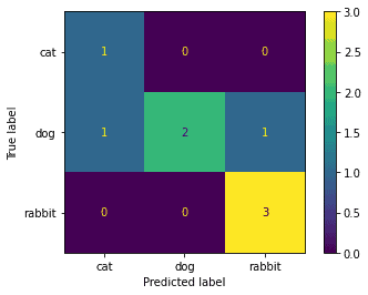 Confusion matrix
You can also find the precision and recall for each of the classes using the following code snippet.
cm_np = np.array(cm)
stats = pd.DataFrame(index=class_labels)
stats['Precision'] = [cm_np[i, i]/np.sum(cm_np[:, i]) for i in range(len(cm_np))]
stats['Recall'] = [cm_np[i, i]/np.sum(cm_np[i, :]) for i in range(len(cm_np))]
stats
 Precision and recall for each class
Note: The results are quite poor since the model was trained using just 30 images per class for just 10 epochs. Train it for longer with more images to get significantly better results.
Notebook for Custom Image Classifier
I’ve compiled the steps I mentioned above into a notebook which you can try running on colab or locally. To run in colab, simply click the “Open in Colab” button below.
Conclusion
That’s it! Hope you found this useful. Feel free to reach out with any questions.
Also, check out my other Computer Vision-related blog posts here if interested.