PARSeq for Scene Text Recognition: A Quick Overview
As I discussed in one of my previous blog posts, PARSeq is one of the best-performing scene text recognition (STR) algorithms at the moment. In this article, I’ll try to give a quick overview of the algorithm.
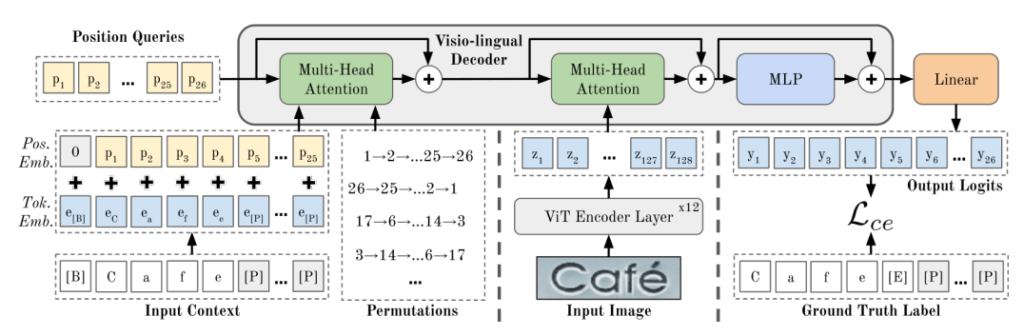 PARSeq model architecture
At a high level, you can break the architecture into 2 main components:
-
Encoder (12 ViT Encoder Layers)
-
Decoder (Visio-lingual Decoder)
The Encoder of PARSeq
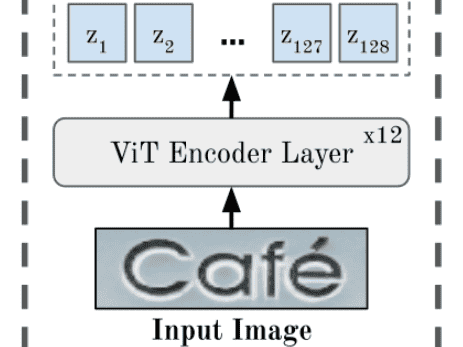 The encoder of PARSeq architecture
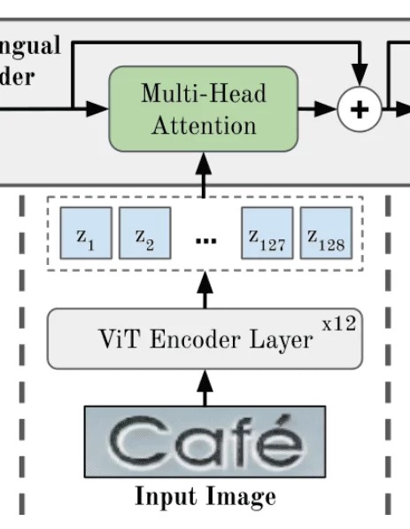
This part is fairly straightforward. The main thing you have to understand here is the Vision Transformer (ViT). Let’s look at the ViT encoder layer as a black box. Accordingly, its input is an image, and the output is a set of vectors, each of which encapsulates details on a certain part of the image. Knowing that should be enough for now. Take a look at the next sub-section below if you want to get a slightly better idea or feel free to skip it if you don’t.
A Quick Summary of Vision Transformers (ViT)
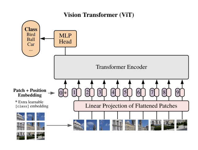 ViT high-level architecture
To put it simply, it is a slight alteration (or rather, an extension) to a regular Transformer that enables it to accept images instead of words or vectors. (Quick Note: Check out this great article on Transformers if you’re not too familiar with it).
First, each image is broken down into sub-images and flattened to obtain a vector. Next, this vector goes into a simple, trainable linear projection layer (multiplied by a trainable matrix). The resulting vectors are combined with the positional embedding (as with regular transformers) and fed into the encoder. The output of the encoder is usually pretrained on a task like classification. Finally, you can fine-tune the model on a preferred downstream task.
ViT in the PARSeq Encoder
Accordingly, ViT generates output vectors (zᵢ) for each sub-image and passes them into the Visio-lingual decoder. Specifically, a Multi-Head Attention (MHA) layer within the decoder. We’ll talk more about this in the next section.
The Decoder of PARSeq
This is where the bulk of the algorithm is. The main novelty behind PARSeq is based on a different model called XLNet.
A Quick Summary of XLNet
It was the first paper that outperformed the BERT model in NLP tasks. Work prior to XLNet had approached the task of natural language understanding by either reading the text from left to right, right to left, or both (as with BERT). XLNet proposed the feeding of different permutations (orders) of words during training. This concept is known as Permutation Language Modeling (PLM).
You may then have the question: how would the model know the order of the letters if it’s shuffled? Turns out, the order in which the letters are fed to the model through positional embeddings remains the same. The only thing that changes is the order in which the model masks the remaining characters. Take a look at this article or this video for a more thorough explanation.
PLM in PARSeq
Similar to XLNet, the usage of PLM in PARSeq benefits both context-aware STR (i.e. images that contain words from a known vocabulary) and context-free STR (i.e. images that may contain undefined words). However, as opposed to a regular Transformer (Transformer-XL to be more specific) in XLNet, PARSeq uses a Vision Transformer (ViT). We’ll talk more about this in the next section.
The 1st Multi-Head Attention Module
Now, let’s pay attention to the left side of the architecture (see what I did there ;-) ).
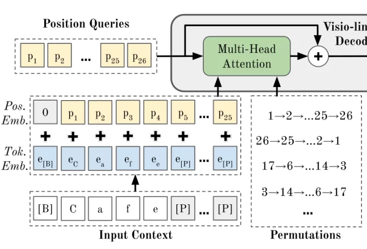 Left part of the PARSeq model architecture
All inputs in this region focus on the Multi-head attention (MHA) module. If you’re not comfortable with MHA yet, then I’d highly recommend reading the article on Transformers I previously mentioned.
-
Positional embeddings / Position queries: This is an encoding of the possible character positions in the input text.
-
Token embedding: This is an encoding of the actual characters in the input text
First, the addition of the position embedding and the token embedding forms the context embedding. Next, this context embedding passes to the Multi-head attention module along with the separate positional embedding. Additionally, the positional embeddings are also passed into the Multi-head attention module separately (shown on the diagram as position queries). Here, the query to the MHA module are the position queries, while both the key and value are denoted by the context embeddings.
Quick Note: As I described in the encoder section, the encoder outputs a z vector for each of the image segments. Thus, if there are d image segments, the output of the encoder would have d vectors. Similarly, all the embeddings I mentioned above would also have d sets, even though they aren’t shown on the architecture.
In addition to these inputs, the MHA module also accepts a list of permutations. These permutations are used in combination with a concept called Look-Ahead Mask. You may have already seen this if you’re familiar with Transformers. Essentially, it is a way to mask the characters in front, to prevent the model from simply “copy pasting” the characters from the input. Let’s discuss a bit about how this works with permutations.
Permutations
Quick Note: As you can probably guess, a string of 25 characters (as denoted in the architecture) would have about 10²⁵ permutations, which is way too high to process. So, the authors use a subset of permutations and their mirrored orders.
To understand how the permutations are accounted for by the MHA, consider the example below, which appeared on the PARSeq paper:
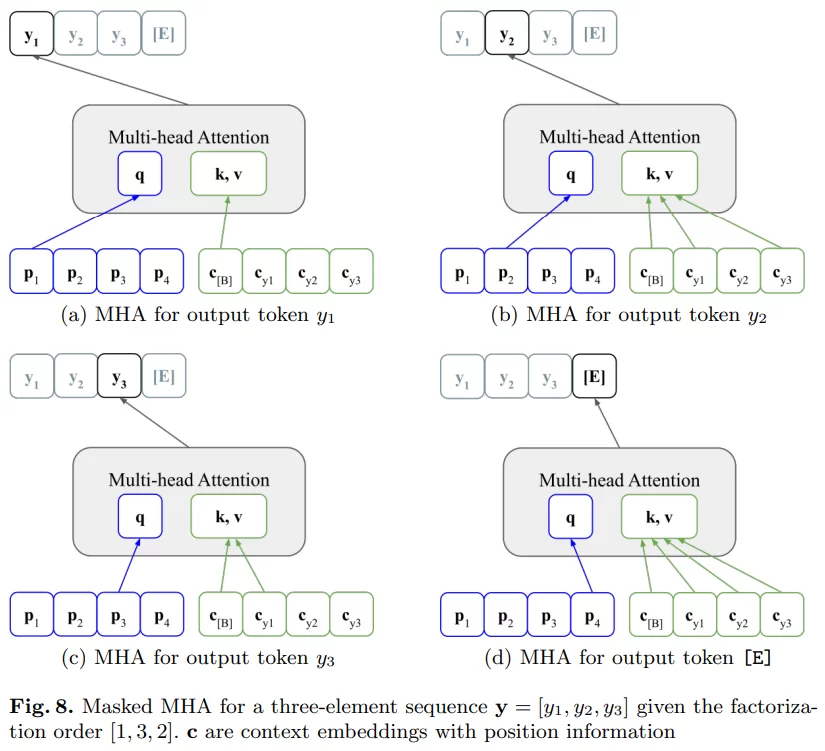 Masked MHA as described in the PARSeq paper
The diagram above considers a string with 3 characters and a permutation of [1, 3, 2] (as opposed to the normal [1, 2, 3]).
Let’s walk through the 4 diagrams in the above image. As we go from (a)->(b)->(c)->(d), we can see that the index of the positional embedding that’s passed increments one by one. This indicates the position of the currently predicted character.
Looking at the permutation ([1, 3, 2]), first, we mask all the characters in front of the position at the first index (1). Thus, only the context of the beginning character (c[B]) is provided. At the second index of the permutation, we have number 3. Therefore, we pass all of c[B], cy1, and cy2 and mask cy3. Finally, we reach the end of the string, so we don’t have to mask anything.
The effect of doing this is that, now, the model is trained for words that may or may not be in the vocabulary, making it more robust.
The 2nd Multi-Head Attention Module
 The 2nd MHA module in PARSeq
Alright, if you understood the previous parts, this part should be fairly easy. Here, the MHA module takes the following inputs:
-
query = Output of the previous MHA module
-
key = value = Output of the encoder
Next, the result of this MHA module passes through a Multi-Layer Perceptron (MLP) and exits the decoder.
The Output
Finally, a linear layer transforms the output to a matrix of size (T + 1 by S + 1), where T is the number of output characters and S is the number of characters in the alphabet.
Summary
-
The architecture has 2 parts: the encoder and the decoder.
-
The encoder breaks the images into equal-sized segments and creates a vector representation of each segment.
- The decoder does the following:
-
The positional information are combined with the textual information (context) using an MHA module.
-
Next, the result of this module is combined with the result of the encoder using another MHA module.
-
- Finally, the result is transformed to the required output using a linear layer